I Made an AI that Learned to Make Music

Recently I posted a video called “AI Learns to Make Music” and I got some people asking me to talk more about how the technical and implementation details of the project. So, this is my response: an in-depth explanation of the architecture.

The cover of the Ramblings of a Transformer, generated by Deep Dream—a deep convolution neural network which finds and emerges patterns in images.

You can listen to an album of curated pieces generated by the AI (plus some samples I call ‘human + AI’—samples generated by the AI which are then reworked by a musician friend of mine, Llyode Sorrow).

• You can watch the video for the results.
• Listen to the Ramblings of a Transformer on Soundcloud.

Background

Introduced by Vaswani, et al. in Attention is All You Need, the transformer is a type of sequence-to-sequece (seq2seq) model that projects the input space, a sequence, into another sequence.

A classical example of seq2seq models is neural machine translation (NMT), where the input sequence is a sequence of words in language and model projects it into a sequence of words, with the same meaning, in language .

A popular model of choice for these sorts of tasks is the Long Short-Term Memory (LSTM) variant of Recurrent Neural Networks (RNNs), which is particularly good at modelling data with long-term dependencies; that is, an LSTM ‘remembers’ particular information (deemed importation) from the past giving it access to a context, and allowing it to make more informed decisions.

Architecture of a Seq2Seq Model

A typical seq2seq model consists of two parts: an embedding, encoder, and a decoder. Before looking at the function of the embedding layer, let’s understand the other main components. The encoder takes in a sequence of dense float-vectors which represent the elements of the sequence and project them into a higher-dimensional vector space. Then, this encoded context vector is fed into a decoder—which as the name suggests, decodes the context vector. Finally, the output is a probability dsitribution over the whole vocabulary, and it specifies which the probability that any word (in the target language) is to come next.

The underlying model of the encoder and decoder is not a concern in the architecture of seq2seq models (though they are typically LSTMs for the reasons mentioned above). This encoder-decoder variant of the seq2seq architecture is also called an autoencoder.

Notice that the autoencoder operates on a continuous vector space, meaning that we need to map our text data into this space. We cannot just feed the neural network characters and expect it to work.

Data Encoding and Word Embeddings

One idea might be to encode words in some discrete vector space. We might define a function $\mathcal{M}(w)$ to generate a unique id for each word in a finite vocabulary. The id function $\mathcal{M}$ has a one-to-one mapping to the raw input sequence of words, $X$, which follows from the definition of the encoded input sequence, $X^\prime=\{x\in X\mid\mathcal{M}(x)\}$, and the fact that $\mathcal{M}$ gives unique ids. While this encoding sequence will work, as it is not a continuous distribution of the vocabulary, the results of the model will be sub-optimal. In specific, representing sequences with integer ids has the major drawback of introducing ordinal relationships into your data due to the inherent ordinal structure of integers—even when there are none.

Instead, we can project this discrete vector space into a truly continuous vector space by using an embedding layer. The embedding layer acts as a lookup table between the input integer event ids and a dense float-vector representation of these. During training, it learns a map which embeds each discrete element in a continuous vector space.

While this concept of projecting discrete spaces into continuous ones might seem to make sense at a high-level, I still think there is a lot of magic going on behind-the-scenes: I mean, after all, what does it even mean for discrete data to become continous? Because of this, I want to take some time at a simpler example, devoid of language, to illustrate the fundamental concept behind discrete-to-continuous vector space mapping.

Movie Rankings

Inspired by the Personality Embedding example from Illustrated Word2Vec.

Suppose that we are building a movie recommendation system, and to feed the movies into a neural network, we first need to represent them in a continous vector space. For each movie, we have a set of attributes:

• Popularity Score: how popular the movie is (0-100).
• Freshness Score: how new the movie is (0-100).
• Comedy Score: how funny the movie is (0-100).
• Action Score: how much action the movie has (0-100).
• Horror Score: how scary the movie is (0-100).
• Revenue
• Budget

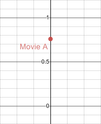
Say we have a movie that scored 76/100 on the popularity metric. We could normalize it to a range of to and plot it on a single axis:

However, this doesn’t really reflect the movie as a whole because it rejects all the other attributes. We cannot really judge the quality of the film solely on its popularity. So, we add another dimension: freshness.

Now we can start to make much better decisions about which film is better to recommend. In this case, while the film might be really popular, it is also really old (since it has a 2/100 in freshness). The actual information behind these metrics is not really important, and they are meaningless, but the point I want to make is that we are continuously updating our vector representation, adding more axes, to get a better understanding of the data.

This vector representation of our movies becomes particularly exciting when we have multiple data points that we’d like to compare. The ability to compare movies becomes really easy in this vector space—which as we can imagine might be very important in designing a recommendation system.

Just visually, we can see that Movie $B$ and Movie $C$ are much more similar to one another than Movie $A$ and Movie $C$, in large part because the angle between $\vec{B}$ and $\vec{C}$ is much smaller than $\vec{A}$ and $\vec{C}$; however, the magnitude of $\vec{A}$ is much closer to $\vec{C}$ than that of $\vec{B}$, so in that respect, is more similar to $\vec{C}$. Thus, we may decide to define a similarity score between two movies as a balance between how similar their magnitudes and directions are. Cosine similarity is this type of measure, which as defined as the cosine of the angle between the two vectors in comparison: $\cos(\theta)$ where $\theta$ is the angle between $\vec{u}$ and $\vec{v}$, the vectors to compare. A cosine similarity of $-1$ means exactly opposite, $1$ means exactly the same, and $0$ means that the two vectors are orthogonal (i.e. perpendicular in two-dimensions).

Following from the definition of cosine similarity and recalling the dot product, $\vec{u}\cdot\vec{v}=\|\vec{u}\|\|\vec{v}\|\cos(\theta)$, the similarity, $S(\vec{u},\vec{v})$, of two movie represented by vectors $\vec{u}$ and $\vec{v}$ is given by

$S(\vec{u}, \vec{v})=\frac{\vec{u}\cdot\vec{v}}{\|\vec{u}\|\|\vec{v}\|},$

which can be generalized to $n$-dimensions as

$S(\vec{u},\vec{v})=\frac{\sum_{k=1}^n u_k v_k}{\sqrt{\sum_{k=1}^n v_k \sum_{k=1}^n u_k}},$

giving us a handy formula for comparing any two movies. Let’s use $S(\vec{u},\vec{v})$ to see how similar Movie $A$ is to Movie $C$, and how similar Movie $B$ is to Movie $C$:

• $S(\vec{A},\vec{C})\approx0.35$
• $S(\vec{B},\vec{C})\approx0.52$

So clearly, our visual analysis was correct: Movie $B$ and Movie $C$ are much more similar—about $1.5$ times more similar than Movie $A$ and Movie $C$.

Of course, we can continue this process: adding more dimensions until we see that there is marginal benefit in including more attributes. For example, we may find that revenue and budget are irrelevant metrics for recommending movies. This process is called Principle Component Analysis (PCA). While we performed it manually, there exist computational approaches as well—though that is not the point here. The point is that an embedding layer is not much different. It takes the data and tries to figure out which attributes best describe the data, and then construct an -dimensional vector space representation of the data. The key difference however is that an embedding layer is not given all these attributes; rather, it is trained on a large corpus to know which words are similar to one another and use that information to best organize the vocabulary it is fed in. One fascinating property of word embeddings is that their representation encodes features such as analogies (see Illustrated Word2Vec).

Hopefully, this example, while crude, has help illuminate what it means to take some discrete data and map it to a continuous vector space.

Attention

The main ingredient of transformers is their attention mechanism which looks at a sequence and at each timestep, focuses only on a part of the sequence, paying more attention to the most important parts of the sequence. Attention is focus. This make sense since after all, language is riddled with a lot of unnecessary information. After all, this is how we read, we pay attention to specific patterns of letters and words, not to the individual letters themselves. It’s why we can read something like:

I cdnuolt blveiee taht I cluod aulaclty uesdnatnrd waht I was rdanieg. The phaonmneal pweor of the hmuan mind!

Aoccdrnig to a rscheearch at Cmabrigde Uinervtisy, it dseno’t mtaetr in waht oerdr the ltteres in a wrod are, the olny iproamtnt tihng is taht the frsit and lsat ltteer be in the rghit pclae.

Applied to a seq2seq autoencoder architecture, the attention mechanism keeps a shortcut of keywords in the sequence, which can then be accessed by the model at any timestep. This is in contrast to an LSTM autoencoder which discards all intermediate states of the encoder, and only initializes the decoder with the final state of the encoder. Attention helps to resolve the issue of long-term dependencies.

Whereas an LSTM autoencoder rapidly degrades in quality as the length of the input sequence increases, a transformer model is much better at modelling these long-term structures since it has access to all past states (thanks to attention)!

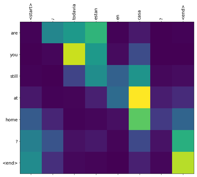
The following plot shows which parts of the input sequence, “are you still at home?”, the model is paying attention to while translating. In particular, the strength of the attention is indicated by the colour of the point (where brighter is better). For example, we see that the model is most of its attention to “you”, “at”, “home”, and “?”, which makes sense since the meaning of the sentence is contained in “you at home?” The rest is merely semantic filler, and doesn’t contribute much to the meaning of the sentence.

What is a transformer, anyway?

For a very detailed explanation, see Jay Alammar’s Illustrated Transformer post.

transformers can be used as the backend in seq2seq models in very much the same way as LSTMs are. However, the key difference between LSTMs and transformers is that the latter have no recurrent neural network components. Due to the attention mechanism of transformers, they don’t need recurrences to remember information and model long-term structure.

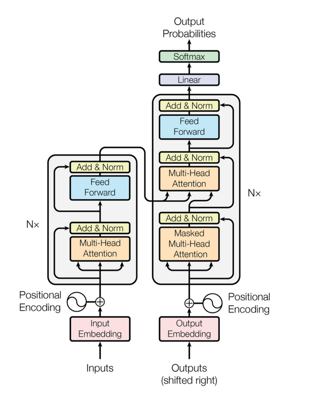A transformer, as outlined in Attention is All You Need, consists of both an encoder and decoder, which can both be stacked on top of one another to increase the capacity of the model. An encoder/decoder layer consists of stacked multi-head attention layers and a feed forward (fully connected) linear layer.

Besides performing input embedding, we also encode the positions of the elements in the sequence since unlike RNNs, transformer don’t maintain past state of how sequences were fed in (rather, attention takes the place of this and stores important information), we encode the position of each element along with its embedding (adding the positonal encoding to the embedding vector). Unlike the input embeddings, the positional encodings are not learned by the model.

The Transformer-Decoder

A very special variant on the transformer model, called a transformer-decoder, allows us to generate text using transformer models. Similar to other language generation models (such as an LSTM text generator), a transformer-Decoder merely consists of stacked decoder layers. OpenAI’s GPT-2 model demonstrated that the higher we stack these layers, the better the results.

How do we generate text?

The mechanics of the model remain the same; however, now, instead of first computing a context vector from the input sequence, we feed the input sequence into a series of decoder layers. The output is a probability distribution over how likely an element in the sequence is to come next. We can sample from this distribution, add it to the input sequence, and repeat the process, until we reach an end of sentence (EOS) token.

We can prompt the model with an input sequence and have it fill in the rest, or we can tell it to generate any it wants by inputting a beginning of sentence (BOS) token.

You can try out a transformer-decoder text generator (GPT-2) here.

Text Generation to Music Generation

It turns out that music is actually very similar to text, and we can employ the same methods use in text generation to generate music using decoder-only transformers.

Representing MIDI files as Sequences of Events

We use the serialization scheme proposed in _This Time with Feeling: Learning Expressive Musical Performance _as the basis of our data encoding. The MIDI note events are converted into a sequence of events from the following vocabulary:

• 128 NOTE_ON events for indicating the start of a note with one of 128 MIDI pitches.
• 128 NOTE_OFF events for indicating the end of a note with one of 128 MIDI pitches.
• 100 TIME_SHIFT events for representing a movement forward in time in 10 ms increment (possible values range from 10 ms to 1 s).
• 32 VELOCITY events for representing the velocity of the next NOTE_ON events in the form of 128 possible MIDI velocities quantized into 32 bins.

For example, consider a simplified scheme where there are only 4 pitches, 10 possible time shift increments, and 4 velocity bins:

• 4 NOTE_ON events for indicating the start of a note with one of 4 pitches.
• 4 NOTE_OFF events for indicating the end of a note with one of 4 pitches
• 10 TIME_SHIFT events for representing a movement in time in 1 ms increment (possible values range from 1 ms to 10 ms).
• 4 VELOCITY events for representing the velocity of the next NOTE_ON events in the form of 128 possible MIDI velocities quantized into 4 bins: 1-32, 33-64, 65-96, 97-128.

In this simplified example, a single step consists of a 22-dimensional one-hot vector. Figure 1 illustrates the structure of one of these vectors and Figure 2 illustrates an example MIDI file encoded as a series of these one-hot vectors.

In the scheme presented by Oore, et al., 2018, the MIDI files are first preprocessed by extending note durations in segments where the sustain pedal is active. The sustain pedal is considered to be active (or down) if it is within a value of less than 64. On the other hand, it is considered to be inactive (or up) if it is above a value of 64. All notes within a period of time where the sustain pedal is active are extended so that they span the entirety of the sustain pedal period or to the start of the next note of the same pitch, whichever happens first. This however, removes the expressiveness that sustain pedals may have on the performance, and it means that there is no way to distinguish note length from sustains in the final output; on the other hand, VSTi plugins and other musical renderers distinguish between these two events—for they are intrinsically separate features. Thus, we introduce two new verbs into the event-based description:

• A SUSTAIN_ON event indicating that the sustain pedal is down.
• A SUSTAIN_OFF event indicating that the sustain pedal is up.

Therefore, with the added sustain events, the whole encoding consists of a 390-dimensional one-hot vector.

The problem with one-hot vectors

Just as we might want to use word embeddings for text sequences, we want to use embeddings for our events. By design, one-hot vectors are sparse vectors which contain a lot of redundancies. As the dimensionality of our data increases, we find that training a model on these one-hot vectors becomes more and more challenging---requiring a substantial amount of GPU memory. Instead, we use the same input embedding and positional encoding used in the original transformer model, and transform our input sequence from one-hot vectors to unique integer ids (these integer ids can be thought of as the index of the ‘hot’ bit in the one-hot vector; for example, if our event one-hot vector is [0, 1, 0, 0] then the event has an id of $1$, since that is the index of the active element in the one-hot vector).

Training the Model

We train the model using a technique called teacher-forcing. This is where the output sequence is shifted by one timestep forward from the input sequence. This means that the model is forced to predict the event at time with only information from timesteps $1$ to $t$ . Thus, at each training step, the input is event $i$ and the target is event $i+1$. Note that since we are effectively shifting the whole sequence by one timestep, we prepend the BOS token to the start of the sequence and append an EOS token to the end of the sequence.

This technique of feeding in the correct input for timestep $t+1$ regardless of the output at timestep $t$ is called teacher-forcing because it is analogous to a teacher feeding the correct answer to a student before moving on to the next problem. The idea being that if a question depends on another, the student can at least have a chance to complete the result of the problems even if they get the last one wrong.

Results

Here’s a curated list of results from both an LSTM and transformer model trained to generate music.

MusicRNN (LSTM variant)

Samples from the LSTM generator were not very good. Some of them had some interesting moments, but they suffered degradation way too quickly to create any usable music.

• Sample 1: Starts strong and very quickly goes into chaos.
• Sample 2: Not really sure what to make of it.
• Sample 3: Not terrible at all, but not very good either.

Transformer

• Sample 1: Minor flaws present within the piece (especially towards the end); however, still very coherent, especially for its length.
• Sample 2: Piece contains two similar distinct parts but an awkward transition between them; however, the parts themselves are very nice.
• Sample 3: Very jazzy!

We recommend you check out the album of curated songs.

Source Code

Wanna experiment with the models yourself? The code is publicly available on GitHub.

‌

‌