How to Use Different Data Visualizations in the Grafana Dashboard

‌

In this post, we will see how to use different visualizations, like the simple graph, pie chart, or world map panel in the Grafana dashboard. We'll do this by writing queries in the Influx query language and fetching data from the InfluxDB database which is a time-series database.

• a. Data Visualization
• b. Installing Plugins Docker Grafana
• c. Writing to the InfluxDB2.0

LINE CHARTS:

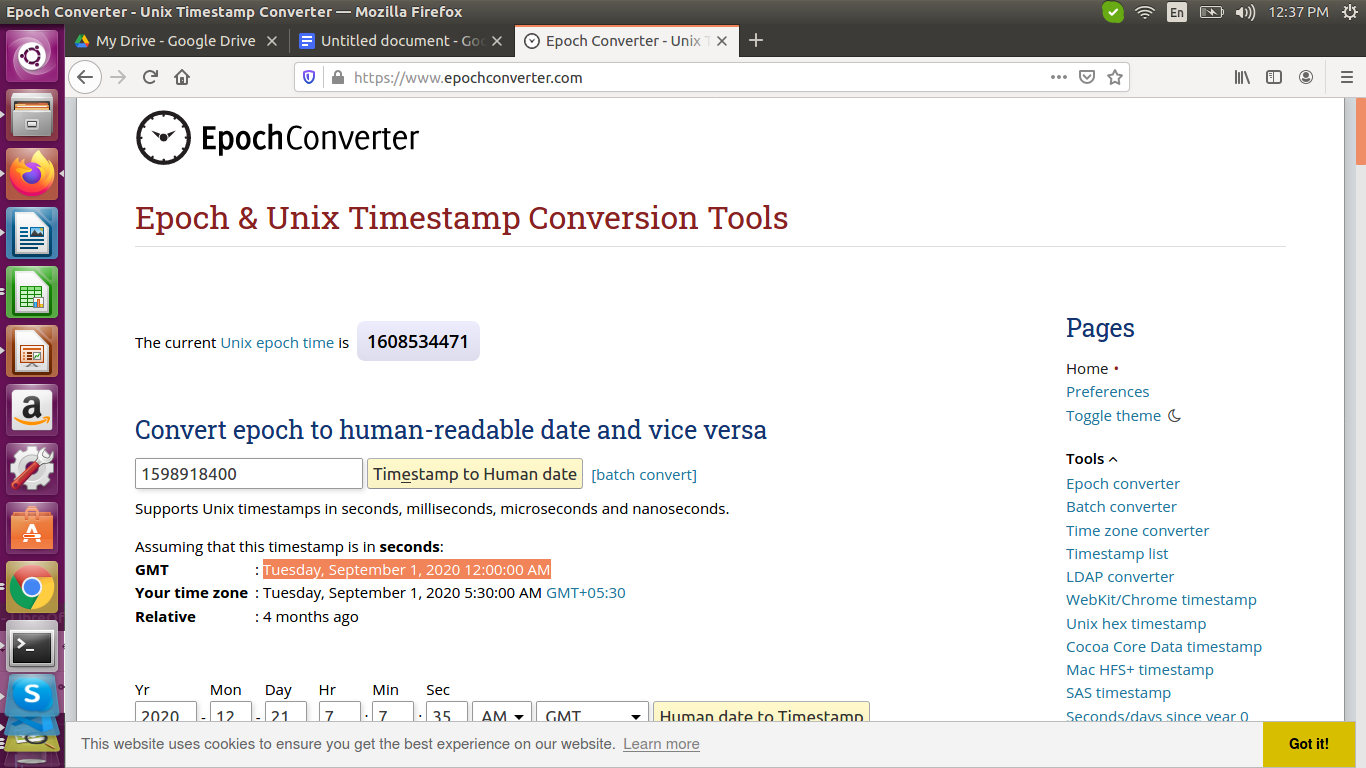
1. As we can see, we are showing the records for 2 different blocks, i.e, DS_Id = 0 and DS_Id = 1.The timestamp is the same for both the blocks, 1598918400, 1598918402, 15989The date for the above can be obtained from the link: https://www.epochconverter.com/

Our requirement is to get the aggregated power for POWER_A, POWER_B, POWER_C fields.

‌

For example, for the timestamp 1598918400:

We have values for POWER_A as 1403.421W and 821.847W, sum as 2225.268W. Likewise, we have to calculate for all the time-series values(1598918402, 1598918403, 1598918404, …) for POWER_A, POWER_B and POWER_C also.

‌

This computation is done in Grafana. We are implementing this using the SQL syntax like queries as shown below:

We are going to compute the aggregated power for the field POWER_A now.

All the queries were constructed and executed successfully by Narendra Reddy Mallidi, SQL Developer.

We have our first query below:

SELECT POWER_A as AA FROM "hdb2" WHERE "DS_ID" = '0'

Here, POWER_A is the variable where are going to fetch from the table(table is called measurement in InfluxDB queries) named "hdb2".

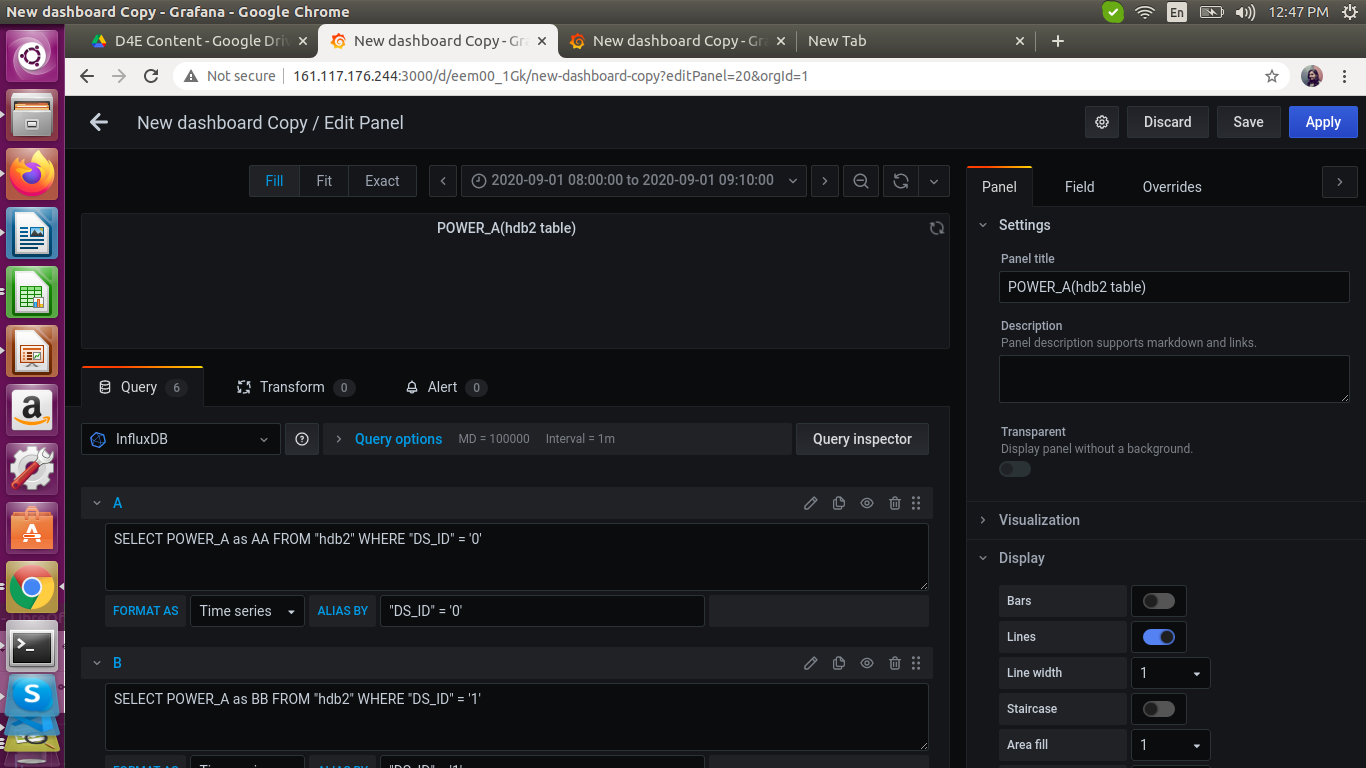The same thing is followed for other 4 blocks also(DS_ID =’1’, DS_ID=’2’, DS_ID=’3’, DS_ID=’4’)

SELECT POWER_A as BB FROM "hdb2" WHERE "DS_ID" = '1'
SELECT POWER_A as CC FROM "hdb2" WHERE "DS_ID" = '2'
SELECT POWER_A as DD FROM "hdb2" WHERE "DS_ID" = '3'
SELECT POWER_A as EE FROM "hdb2" WHERE "DS_ID" = '4'

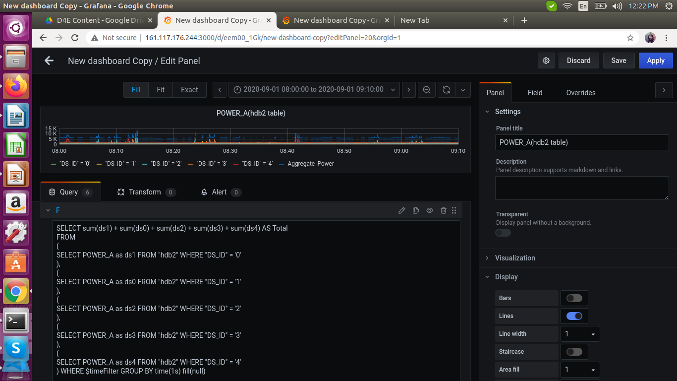
Now, we compute the aggregated power for POWER_A with the below query:

SELECT sum(ds1) + sum(ds0) + sum(ds2) + sum(ds3) + sum(ds4) AS Total
FROM
(
SELECT POWER_A as ds0 FROM "hdb2" WHERE "DS_ID" = '0'
),
(
SELECT POWER_A as ds1 FROM "hdb2" WHERE "DS_ID" = '1'
),
(
SELECT POWER_A as ds2 FROM "hdb2" WHERE "DS_ID" = '2'
),
(
SELECT POWER_A as ds3 FROM "hdb2" WHERE "DS_ID" = '3'
),
(
SELECT POWER_A as ds4 FROM "hdb2" WHERE "DS_ID" = '4'
) WHERE $timeFilter GROUP BY time(1s) fill(null)

Here, hdb2 is the table name in our INFLUXDB1.8 database from where we are fetching our data into the Grafana dashboard running at port 3000.

We get the graph as shown below:

TIMESTAMP	SAMPLE	POWER_A
2020-09-01 08:27:16	Sample 1	7.92k

TIMESTAMP	SAMPLE	POWER_A
2020-09-01 08:17:08	Sample 2	5.77k

‌

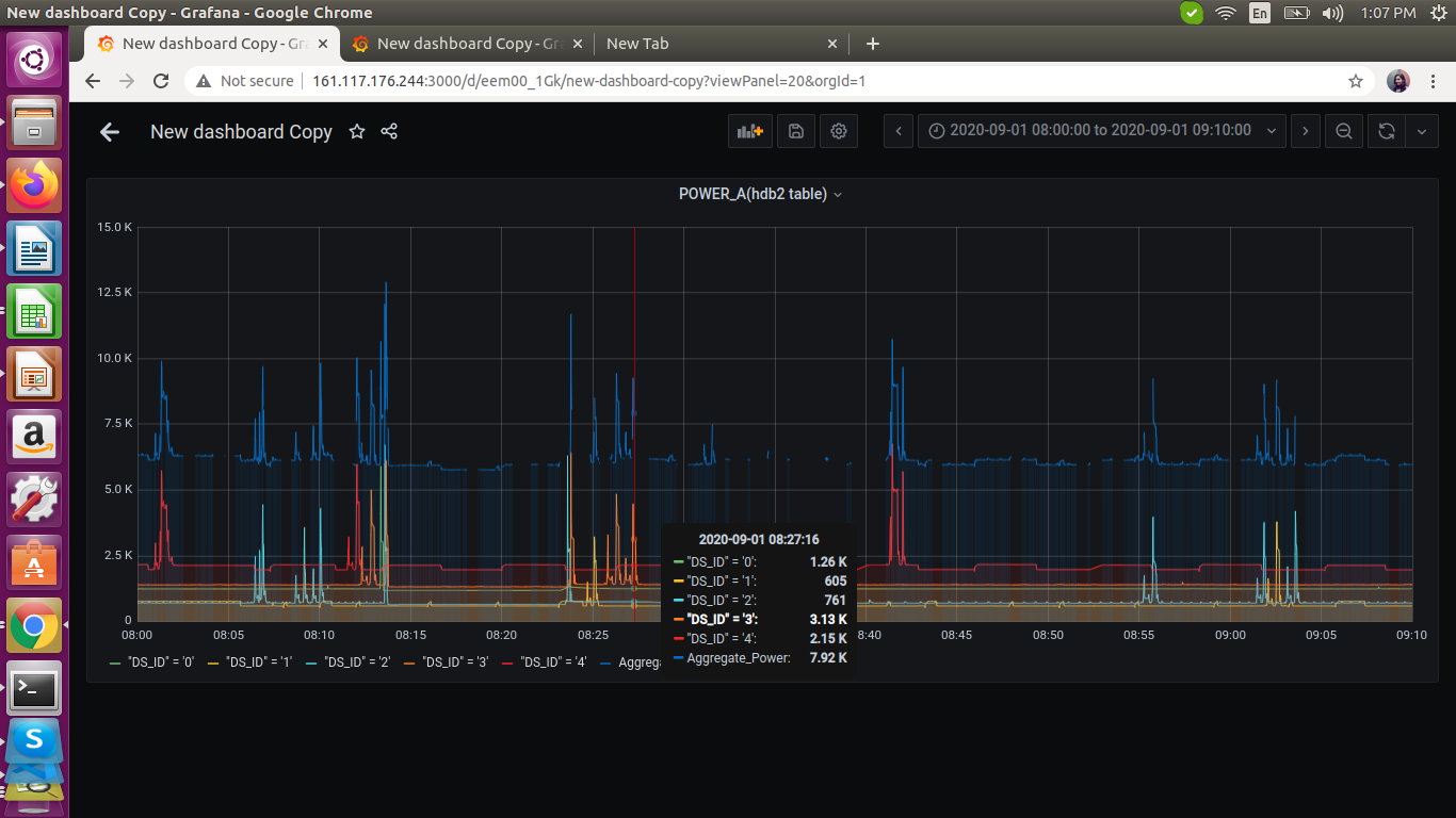
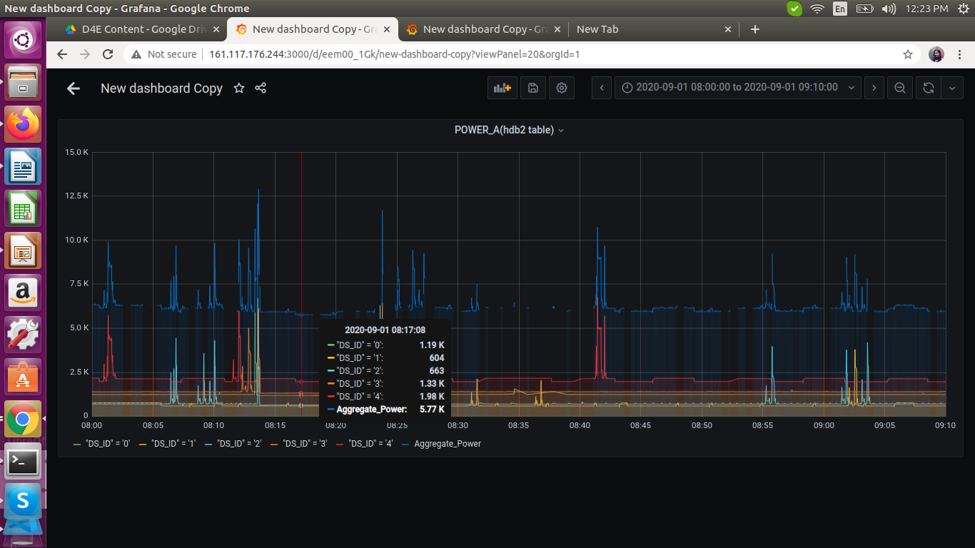We are getting the correct aggregated values for POWER_A. We need to do the same for POWER_B and POWER_C.

For POWER_B:

SELECT sum(ds1) + sum(ds0) + sum(ds2) + sum(ds3) + sum(ds4) AS PB
FROM
(
SELECT POWER_B as ds1 FROM "hdb2" WHERE "DS_ID" = '1'
),
(
SELECT POWER_B as ds0 FROM "hdb2" WHERE "DS_ID" = '0'
),
(
SELECT POWER_B as ds2 FROM "hdb2" WHERE "DS_ID" = '2'
),
(
SELECT POWER_B as ds3 FROM "hdb2" WHERE "DS_ID" = '3'
),
(
SELECT POWER_B as ds4 FROM "hdb2" WHERE "DS_ID" = '4'
) WHERE $timeFilter GROUP BY time(1s) fill(null)

For POWER_C:

SELECT sum(ds1) + sum(ds0) + sum(ds2) + sum(ds3) + sum(ds4) AS PC
FROM
(
SELECT POWER_C as ds1 FROM "hdb2" WHERE "DS_ID" = '1'
),
(
SELECT POWER_C as ds0 FROM "hdb2" WHERE "DS_ID" = '0'
),
(
SELECT POWER_C as ds2 FROM "hdb2" WHERE "DS_ID" = '2'
),
(
SELECT POWER_C as ds3 FROM "hdb2" WHERE "DS_ID" = '3'
),
(
SELECT POWER_C as ds4 FROM "hdb2" WHERE "DS_ID" = '4'
) WHERE $timeFilter GROUP BY time(1s) fill(null)

We will get the graph as shown below:

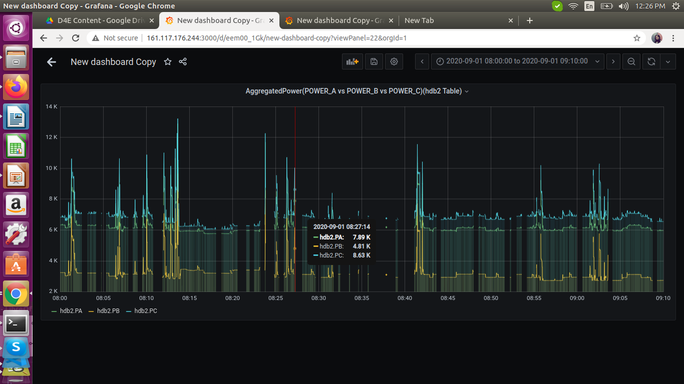
|TIMESTAMP SAMPLE POWER_A

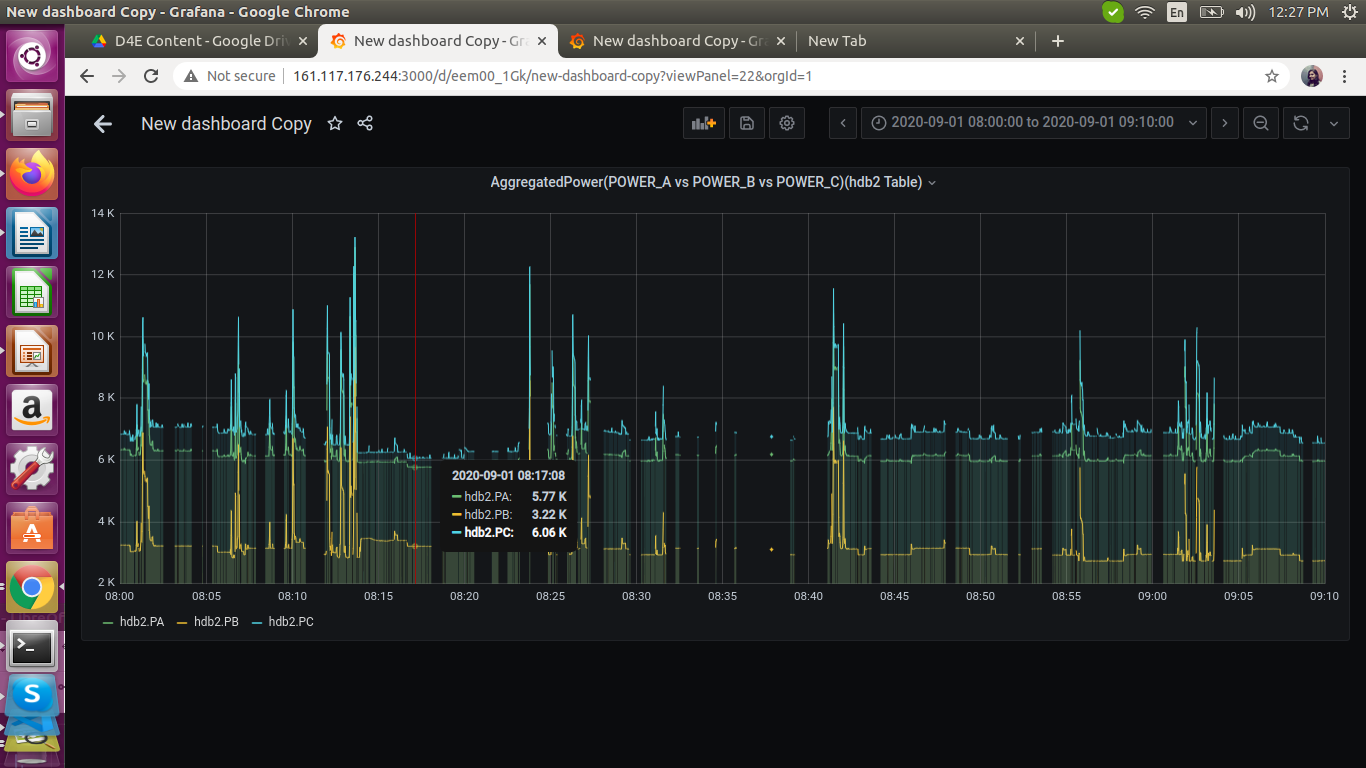
TIMESTAMP	SAMPLE	POWER_A
2020-09-01 08:17:08	Sample 4	5.77k

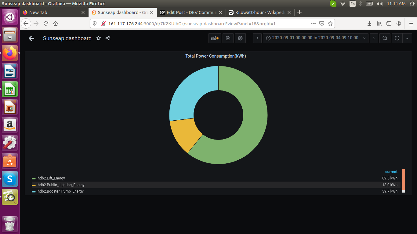
PIE CHART VISUALIZATION:

Below is the query for visualization of 3 components:

‌

Lift_Energy, Public_Lighting_Energy, Booster_Pump_Energy.

SELECT
(( (sum("LIFT_TOTAL")) / (($to - $from) / 1000) ) )* (($to - $from) / 3600000)
as Lift_Energy,
(((sum("LIGHT_TOTAL")) / (($to - $from) / 1000))) * ((($to - $from) / 1000) / 3600)
as Public_Lighting_Energy,
(((sum("PUMP_TOTAL")) / (($to - $from) / 1000))) * ((($to - $from) / 1000) / 3600) as Booster_Pump_Energy
FROM "hdb2" WHERE $timeFilter GROUP BY time(24h)

Here, we have combined 3 subqueries.

(sum("LIFT_TOTAL")) / (($to - $from) / 1000) ) )* (($to - $from) / 3600000) as Lift_Energy

(sum("LIGHT_TOTAL")) / (($to - $from) / 1000))) * ((($to - $from) / 1000) / 3600) as Public_Lighting_Energy

(sum("PUMP_TOTAL")) / (($to - $from) / 1000))) * ((($to - $from) / 1000) / 3600) as Booster_Pump_Energy

All the 3 queries are similar. We will take 1st query. The records are taken for each second,i.e, for every consecutive second we are recording the data. Here, (sum("LIFT_TOTAL")) is the sum computed over the period mentioned - (($**to - $**from) in the time window.

SELECT 
((    (sum("LIFT_TOTAL"))  / ((1599190800000 - 1598898600000) / 1000) ) )* ((1599190800000 - 1598898600000) /  3600000)
as Lift_Energy,
(((sum("LIGHT_TOTAL"))  / ((1599190800000 - 1598898600000) / 1000))) * (((1599190800000 - 1598898600000) / 1000) / 3600)
as Public_Lighting_Energy,
(((sum("PUMP_TOTAL"))  / ((1599190800000 - 1598898600000) / 1000))) * (((1599190800000 - 1598898600000) / 1000) / 3600) as Booster_Pump_Energy
FROM "hdb2" WHERE time >= 1598898600000ms and time <= 1599190800000ms GROUP BY time(24h)

Since the precision is in milliseconds, we are dividing it by 1000.Now, we get total power for the time range applied. The unit for energy consumption is watt-hour(Wh). Example, a 40-watt electric appliance operating continuously for 25 hours uses one kilowatt-hour. The value ((($__to - \_\_from\) / 1000\) / 3600\) gives the total operating hours which multiplied with the total power,i.e,\(sum\("PUMP\_TOTAL"\)\) / \(\(__to - $__from) / 1000))) gives power consumption in watt-hour units.

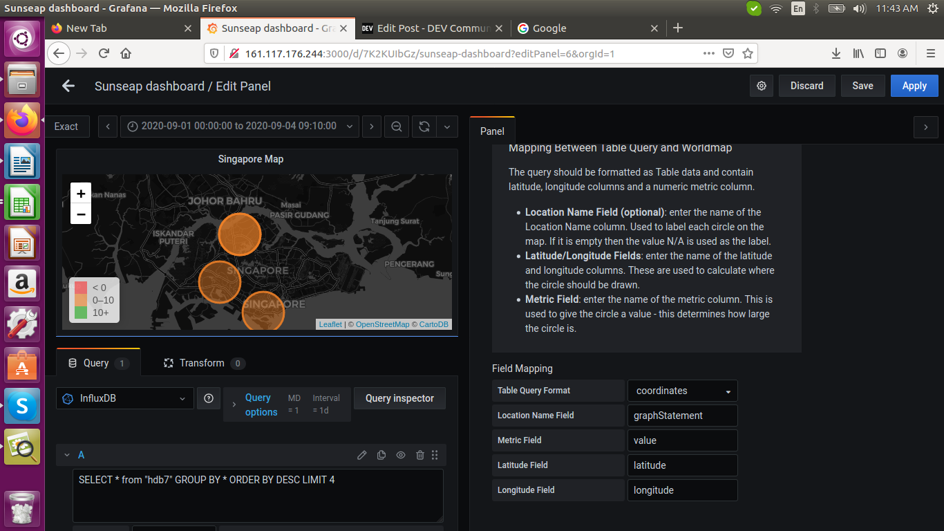
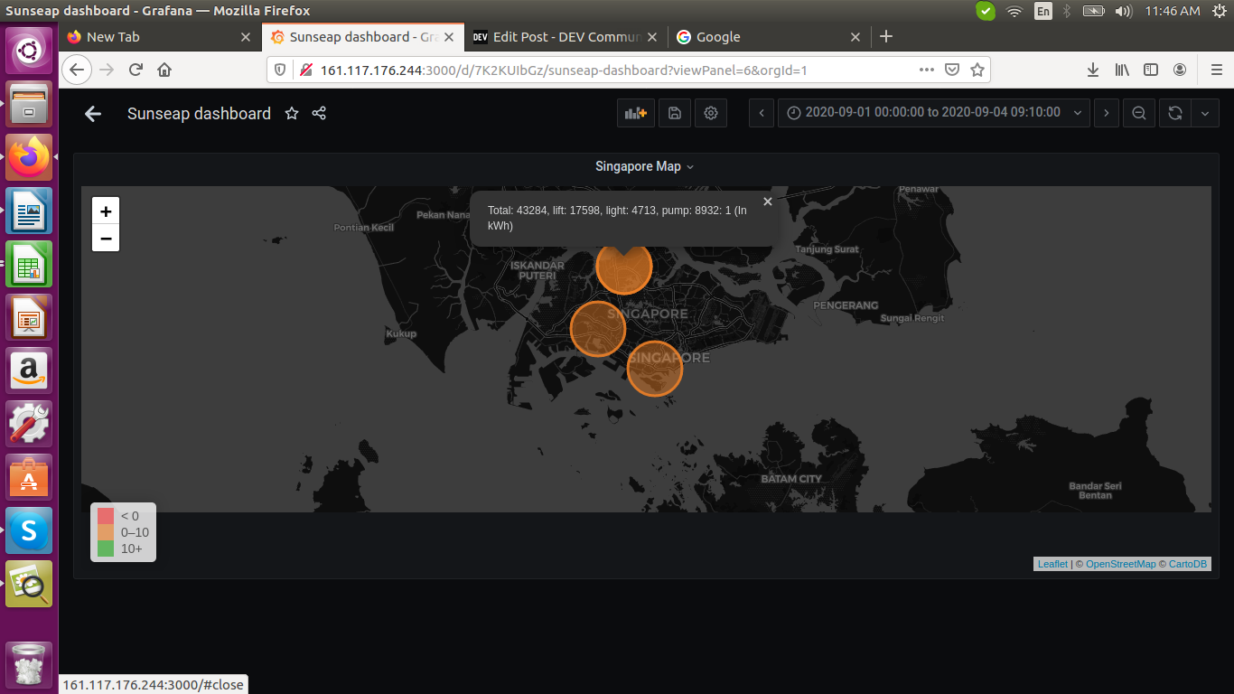
WORLD MAP VISUALIZATION:

‌

The sample csv table we are using for the world map is shown below.

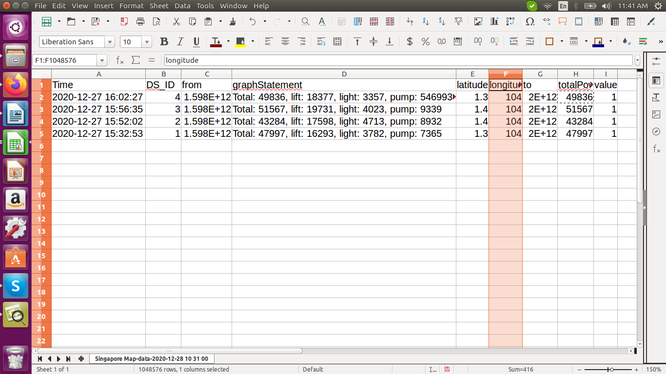
Above is the csv file which we are uploading in the influxdb into the "hdb7" measurement.

Query for world map:

SELECT * from "hdb7" GROUP BY * ORDER BY DESC LIMIT 4

We can see the query and the settings also in the image below. Here, we are using latitude and longitude values to plot the map and put the graphStatement field in the label of the map.

b. More on Installing Plugins Docker Grafana:

Open the SSH terminal on your machine and run the following command:

ssh your_username@host_ip_address

If the username on your local machine matches the one on the server you are trying to connect to, you can just type:

ssh host_ip_address

And hit Enter.

After successful login, execute the below commands in the shell:

sudo docker ps -a
sudo docker exec -it --user=root grafana /bin/sh
grafana-cli plugins install grafana-worldmap-panel
sudo docker container stop d1ead747ec87
sudo docker start d1ead747ec87

1.The command

 sudo docker ps -a

lists all the running containers.

2.

We can execute/test the commands for the application running inside the container with

sudo docker exec -it --user=root grafana /bin/sh

command.

We can also ping to test the port connections with the commands:

curl http://localhost:3000

curl http://160.100.100.204:3000

where the ip-address is of the remote virtual machine provisioned in the cloud which we have logged into.

3.

The plugins are installed with

grafana-cli plugins install grafana-worldmap-panel. 

4.

The docker conatiners are restarted with commands:

 sudo docker container stop d1ead747ec87

sudo docker start d1ead747ec87

   
Last login: Fri Dec 18 19:37:21 2020 from 49.206.11.161
root@d4eViz:~# sudo docker ps -a
CONTAINER ID        IMAGE               COMMAND             CREATED             STATUS              PORTS                    NAMES
d1ead747ec87        grafana/grafana     "/run.sh"           46 hours ago        Up 17 hours         0.0.0.0:3000->3000/tcp   grafana
root@d4eViz:~# sudo docker exec -it --user=root grafana /bin/sh
/usr/share/grafana # grafana-cli plugins install grafana-worldmap-panel
installing grafana-worldmap-panel @ 0.3.2
from: https://grafana.com/api/plugins/grafana-worldmap-panel/versions/0.3.2/download
into: /var/lib/grafana/plugins

✔ Installed grafana-worldmap-panel successfully 

Restart grafana after installing plugins . 

/usr/share/grafana # sudo docker container stop d1ead747ec87
/bin/sh: sudo: not found
/usr/share/grafana # root@d4eViz:~# 
root@d4eViz:~# sudo docker container stop d1ead747ec87
d1ead747ec87
root@d4eViz:~# sudo docker start d1ead747ec87
d1ead747ec87
root@d4eViz:~# 

root@d4eViz:~# sudo docker rm -fv $(sudo docker ps -aq)
08d6b4e38932
root@d4eViz:~# sudo docker run -d -p 3000:3000 --name=grafana -v grafana-storage:/var/lib/grafana grafana/grafana
d1ead747ec87a566c5f8de5c36a705d3b8e1860f7e7dc78b2ea5bf2ef0f574d8
root@d4eViz:~# sudo docker ps -a
CONTAINER ID        IMAGE               COMMAND             CREATED             STATUS              PORTS                    NAMES
d1ead747ec87        grafana/grafana     "/run.sh"           4 seconds ago       Up 4 seconds        0.0.0.0:3000->3000/tcp   grafana
root@d4eViz:~# sudo docker exec -it grafana /bin/sh
/usr/share/grafana $ curl http://localhost:3000
/bin/sh: curl: not found
/usr/share/grafana $ apk add curl
ERROR: Unable to lock database: Permission denied
ERROR: Failed to open apk database: Permission denied
/usr/share/grafana $ root@d4eViz:~# 
root@d4eViz:~# sudo docker exec -it --user=root grafana /bin/sh
/usr/share/grafana # apk add curl
fetch http://dl-cdn.alpinelinux.org/alpine/v3.12/main/x86_64/APKINDEX.tar.gz
fetch http://dl-cdn.alpinelinux.org/alpine/v3.12/community/x86_64/APKINDEX.tar.gz
(1/3) Installing nghttp2-libs (1.41.0-r0)
(2/3) Installing libcurl (7.69.1-r3)
(3/3) Installing curl (7.69.1-r3)
Executing busybox-1.31.1-r19.trigger
Executing glibc-bin-2.30-r0.trigger
/usr/glibc-compat/sbin/ldconfig: /usr/glibc-compat/lib/ld-linux-x86-64.so.2 is not a symbolic link

OK: 27 MiB in 37 packages
/usr/share/grafana # curl http://localhost:3000
Found.

/usr/share/grafana # curl http://160.100.100.204:3000
Found.

/usr/share/grafana # 

c. Writing to the InfluxDB2.0

‌

Reference:https://john.soban.ski/refactor-python-to-influx-2.html

‌

Requirements:

‌

Get started with InfluxDB 2.0

The InfluxDB 2.0 time series platform is purpose-built to collect, store, process and visualize metrics and events. Get started with InfluxDB OSS v2.0 by downloading InfluxDB, installing the necessary executables, and running the initial setup process.

‌

If not installed, follow the link

https://docs.influxdata.com/influxdb/v2.0/get-started/

‌

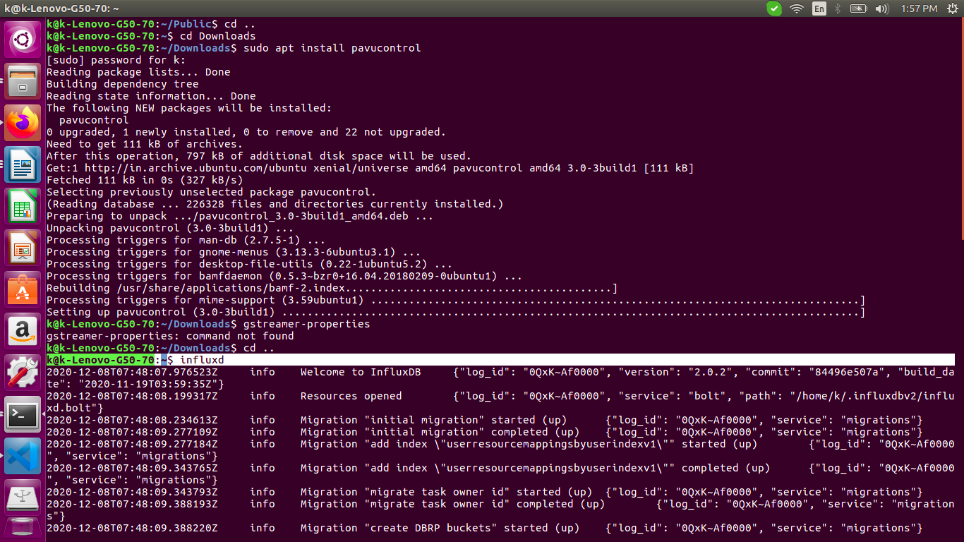
Start InfluxDB by running the influxd daemon:

k@k-Lenovo-G50-70:~$ influxd

Steps:

1. Replace the values of INFLUX_TOKEN, ORG, BUCKET_NAME and measurement_name with the name of the table you need to create.

Also replace the csv path you need to upload the csv file at line:

with open\('/home/k/Downloads/influxData/data\_0\_20200901.csv'\) as csv\_file:

In the csv file, we have time stored in Unix Timestamp format.

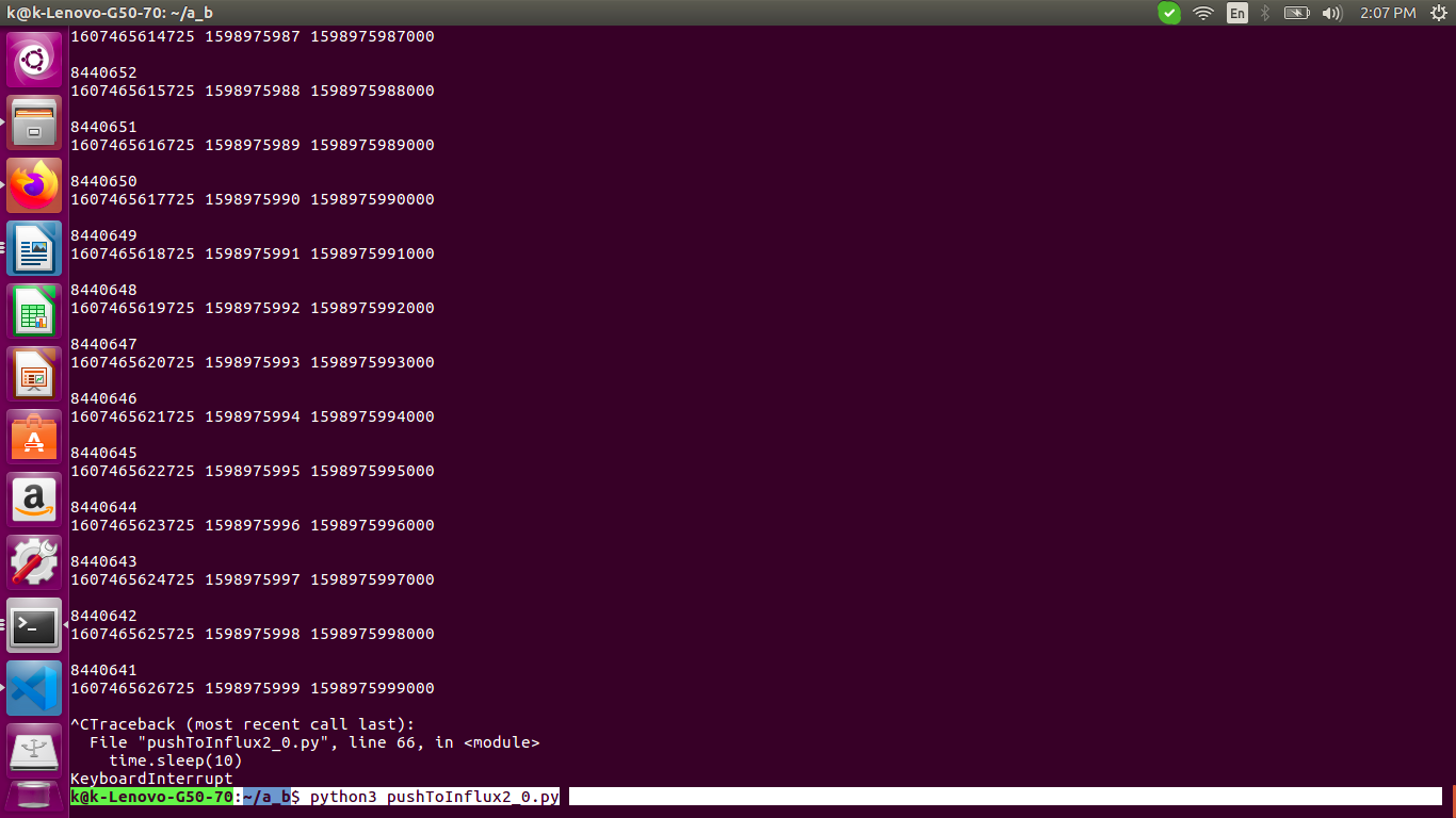
2. Run the below program:

k@k-Lenovo-G50-70:~/a_b$ python3 pushToInflux2_0.py

'''
!/usr/bin/python
'''
import requests
import uuid
import random
import time
import sys
import csv
import json

INFLUX_TOKEN='qCAYOyvOErIP_KaJssk_neFar-o7PdvHL64eWYCD_ofywR_J3iubktdB58A3TE-6sM7C61Gt8qOUPvc4t0WVBg=='
ORG="asz"
INFLUX_CLOUD_URL='localhost'
BUCKET_NAME='b'
'''
Be sure to set precision to ms, not s
'''
QUERY_URI='http://{}:8086/api/v2/write?org={}&bucket={}&precision=ms'.format(INFLUX_CLOUD_URL,ORG,BUCKET_NAME)
headers = {}
headers['Authorization'] = 'Token {}'.format(INFLUX_TOKEN)
measurement_name = 'data_0_20200901'
'''
Increase the points, 2, 10 etc.
'''
number_of_points = 1000
batch_size = 1000

with open('/home/k/Downloads/influxData/data_0_20200901.csv') as csv_file:
    csv_reader = csv.reader(csv_file, delimiter=',')
    print('Processed')
for row in csv_reader:
    _row = 0
    if row[0] == "TIMESTAMP":
        pass
    else:
        _row = int((int(row[0])) * 1000)
    print(_data_end_time, row[0],_row, '\n')
    data.append("{measurement},location={location} POWER_A={POWER_A},POWER_B={POWER_B},POWER_C={POWER_C} {timestamp}"
        .format(measurement=measurement_name, location="reservoir", POWER_A=row[2], POWER_B=row[3], POWER_C=row[4], timestamp=_row))

count = 0
if name == 'main':
  # Check to see if number of points factors into batch size
  count = 0
  if (  number_of_points % batch_size != 0 ):
    raise SystemExit( 'Number of points must be divisible by batch size' )
  # Newline delimit the data
  for batch in range(0, len(data), batch_size):
    time.sleep(10)
    current_batch = '\n'.join( data[batch:batch + batch_size] )
    print(current_batch)
    r = requests.post(QUERY_URI, data=current_batch, headers=headers)
    count = count + 1
    print(r.status_code, count, data[count])

In the InfluxDB2.0 screen page at: http://localhost:8086/orgs/772821f18f2f7a0d/data-explorer?bucket=b

Under the Explore option

We need to set the WINDOW PERIOD as 15s / 1m to see more points on the dashboard.

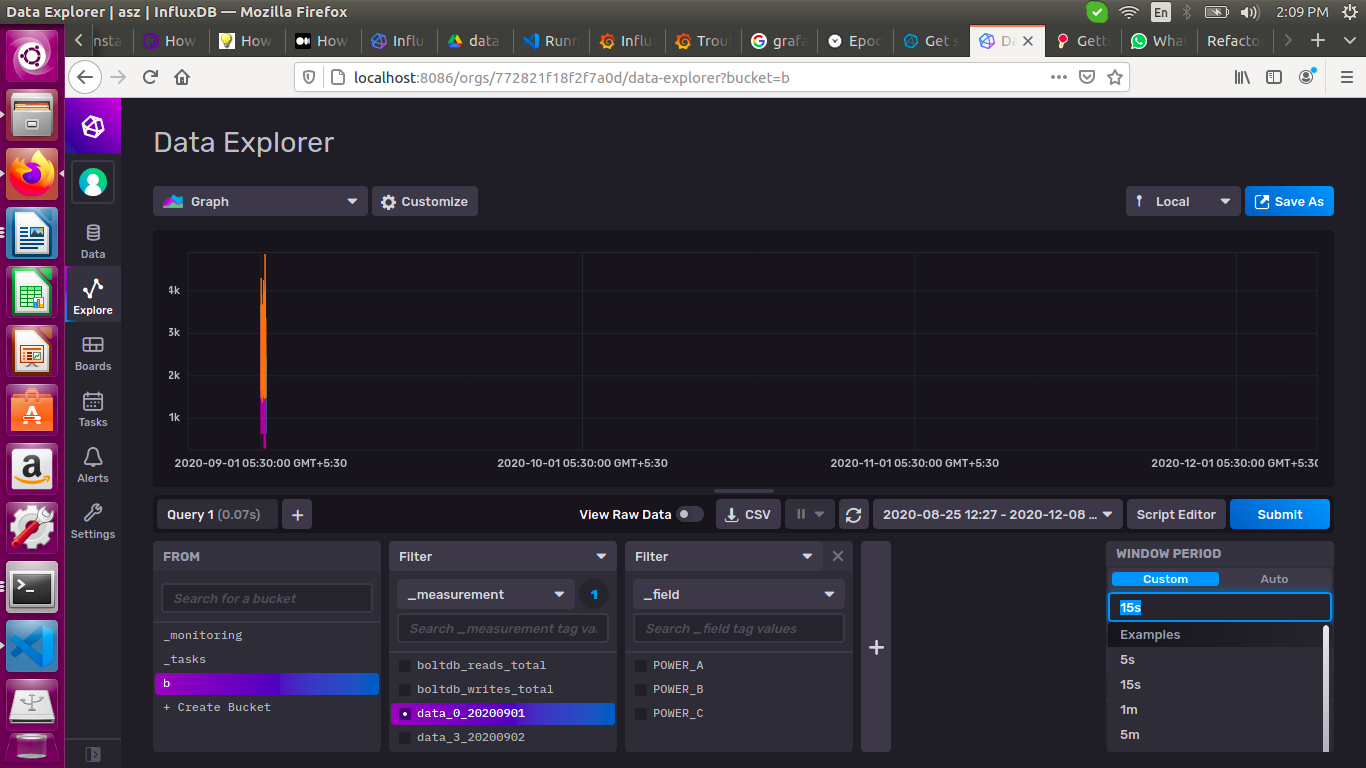
Also, the timing window must be adjusted according to the timestamp of the record.

‌

For example:

So, we need to apply the time range from the above date for the results to show as in the above window.

My Github Profile for code:

Please see the master branch in my repo: https://github.com/krishnakurtakoti/python-influxdb-2.0-write

Also published at https://dev.to/krishnakurtakoti/grafana-dashboard-5f8